Excerpt

This post implements R code to estimate the Rotated Nelson-Siegel yield curve model of Nyholm (2018).

Rotated Nelson-Siegel model

Nyholm (2018) introduced the Rotated Dynamic Nelson-Siegel (RDNS) model with the intention of enhancing the interpretability of yield factors through a more conventional framework. The primary emphasis of this model centers on the short rate component.

Since the factor loading matrix is the key distinguishing difference between DNS and RDNS models, I opt for the period-by-period OLS estimation of the Rotated Nelson-Siegel model for simplicity, rather than the Rotated DNS model.

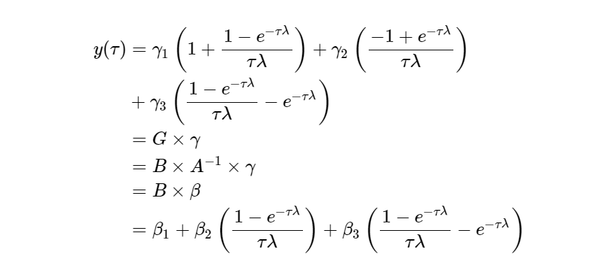
The well-known Nelson-Siegel (NS) model has the following form (B is the NS factor loading matrix).

In order to rotate the NS factors from [Level, -Slope, Curvature] into [Short Rate, Slope, Curvature], the NS model is augmented with a rotation matrix, denoted by A, which is chosen in such a way that the desired factor-interpretation emerges, and such that I=A−¹A, where I is the identity matrix.

Absolutely, keep in mind that the slope factor is defined as the difference between the long-term and short-term components: slope = long-term – short-term.

In sum, the rotation matrix A turns the NS yield factors into RNS yield factors as follows.

Nyholm (2018) rotates the factor structure to enable direct parametrization of the short rate process.

Hence, the RDNS model shares identical statistical properties with the DNS model, rendering it observationally equivalent to the DNS model.

NS and Rotated NS model

The following R code estimates the NS and Rotated NS models by using the period-by-period OLS estimation.

#========================================================#
# Quantitative ALM, Financial Econometrics & Derivatives 
# ML/DL using R, Python, Tensorflow by Sang-Heon Lee 
#
# https://shleeai.blogspot.com
#--------------------------------------------------------#
# Nyholm (2018) Rotated Nelson-Siegel Model
#========================================================#
 
graphics.off(); rm(list = ls())
 
setwd('D:/SHLEE/blog/R/Rotated_NS')
 
# data is located in the following address
# 'https://github.com/Financial-Times/yield-curve-sonification/blob/7d131970377380f118fb9a0e1626f5ed1ecd35ca/yield-curve-monthly-data.csv'
 
yield <- as.matrix(read.csv('yield-curve-monthly-data.csv')[,-1])
mat <- c(1, 3, 6, 12,  24, 36, 60, 84, 120, 240, 360)
 
vcol <- c("darkgray", "blue", "hotpink")
 
#-----------------------------------------------------------
# NS and Rotated NS models
#-----------------------------------------------------------
 
# Factor loading matrix
NS_factor_loading <-function(la, m) {
    B <- cbind(
        rep(1,length(m)), 
        (1-exp(-la*m))/(la*m), 
        (1-exp(-la*m))/(la*m)-exp(-la*m))
    return(B)
}
RNS_factor_loading  <-function(la, m) {
    
    # short rate, conventional slope, curvature
    A1 <- c(1, 1, 0)
    A2 <- c(0,-1, 0)
    A3 <- c(0, 0, 1)
    A <- matrix(cbind(A1, A2, A3), 3, 3, byrow = TRUE)
    G <- NS_factor_loading(la, m)%*%solve(A)
    return(G)
}
 
# fitted yield curve
fit_NS  <- function(beta, la, m)    { 
    return(NS_factor_loading(la, m)%*%beta) 
}
fit_RNS  <- function(gamma, la, m)    { 
    return(RNS_factor_loading(la, m)%*%gamma) 
}
 
# RMSE
rmse_NS <- function(beta, la, y, m) { 
    return(sqrt(mean((y - fit_NS(beta, la, m))^2)))
}
rmse_RNS <- function(gamma, la, y, m) { 
    return(sqrt(mean((y - fit_RNS(gamma, la, m))^2)))
}
 
# Cross-sectional OLS
est_NS_ols <- function(la, y, m) {
    B    <- NS_factor_loading(la, m)
    beta <- solve(t(B)%*%B)%*%t(B)%*%y; 
    rmse <- rmse_NS(beta, la, y, m)
    return(list(beta=beta, la=la, rmse=rmse))
}
est_RNS_ols <- function(la, y, m) {
    G    <- RNS_factor_loading(la, m)
    gamma <- solve(t(G)%*%G)%*%t(G)%*%y; 
    rmse <- rmse_RNS(gamma, la, y, m)
    return(list(gamma=gamma, la=la, rmse=rmse))
}
 
# period-by-period OLS Estimation
est_NS_ols_ts <- function(la, y_all, m) {
    nobs <- nrow(y_all); nmat <- length(m)
    rmse <- rep(NA,nobs)
    beta <- matrix(NA, nobs, 3)
    
    for(t in 1:nobs) {
        lt <- est_NS_ols(la,y_all[t,],m)
        beta[t,] <- lt$beta; rmse[t]  <- lt$rmse
    }
    return(list(beta=beta, la=la, rmse=rmse))
}
est_RNS_ols_ts <- function(la, y_all, m) {
    nobs <- nrow(y_all); nmat <- length(m)
    rmse <- rep(NA,nobs)
    gamma <- matrix(NA, nobs, 3)
 
    for(t in 1:nobs) {
        lt <- est_RNS_ols(la,y_all[t,],m)
        gamma[t,] <- lt$gamma; rmse[t]  <- lt$rmse
    }
    return(list(gamma=gamma, la=la, rmse=rmse))
}
 
 
# Estimation
out_NS  <- est_NS_ols_ts (0.0609, yield, mat)
out_RNS <- est_RNS_ols_ts(0.0609, yield, mat)
 
# plot
x11(width = 16/2, height = 9/2.3)
matplot(out_NS$beta, type="l", lty=1, lwd=4, col = vcol,
        main = paste0("NS model : Avg. RMSE = ", 
                      round(mean(out_NS$rmse),4)))
legend("bottomright", pch = 16, col = vcol, cex = 0.9,
       bty = "n", legend=c("Level","-Slope","Curvature"))
 
x11(width = 16/2, height = 9/2.3)
matplot(out_RNS$gamma, type="l", lty=1, lwd=4, col = vcol,
        main = paste0("Rotated NS model : Avg. RMSE = ", 
                      round(mean(out_RNS$rmse),4)))
legend("bottomright", pch = 16, col = vcol, cex = 0.9,
       bty = "n", legend=c("Short Rate","Slope","Curvature"))

Visit SHLee AI Financial Model to read the full article.